data
|
A data frame, tibble, or data.table.
|
estimate
|
Column name (string) for point estimates.
|
lower
|
Column name (string) for lower confidence interval bounds.
|
upper
|
Column name (string) for upper confidence interval bounds.
|
label
|
Column name (string) for row labels displayed on the y-axis or in the left text panel. If NULL, row numbers are used.
|
group
|
Column name (string) for a grouping variable. Rows that share a group value receive the same colour, and a legend is drawn automatically.
|
is_summary
|
Column name (string) of a logical vector. Rows where this is TRUE are drawn as filled diamonds (e.g. pooled or overall estimates) rather than squares with whiskers.
|
weight
|
Column name (string) of numeric row weights. When provided, point size scales as cex * sqrt(weight / max(weight)), so rows with larger weights appear with a bigger marker. Weights for summary rows are ignored (diamond size is fixed by cex).
|
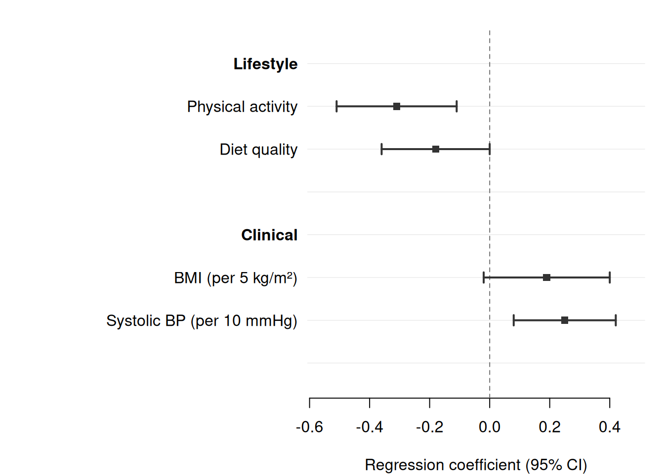
section
|
Column name (string) for a grouping variable that determines section structure. Whenever the value of this column changes (run-length boundary), a bold section header row is automatically inserted before the group. Row order is preserved; no automatic sorting is applied. See also section_indent, section_spacer, and section_cols.
|
subsection
|
Column name (string) for a second-level grouping variable. Requires section. Inserts indented sub-headers beneath each section header. See also subsection_cols.
|
section_indent
|
Logical. If TRUE (default), label values of data rows within a section are automatically indented by two spaces (four spaces for rows within a subsection).
|
section_spacer
|
Logical. If TRUE (default), a blank spacer row is appended after the last row of each section.
|
section_cols
|
Named character vector. Names must be a subset of the names of cols. Values are column names in data whose first non-NA entry in each section is shown in that section’s header row. Columns not listed here display ““ in the header row. Use this to show section-level summaries (e.g. ”k = 3 studies”) next to the section header.
|
subsection_cols
|
Like section_cols but for subsection header rows.
|
ref_label
|
Logical. When TRUE and section is provided, rows with NA estimates that are present in the original data (i.e. reference category rows, not auto-generated headers) have ” (Ref.)“ appended to their label. Default is FALSE.
|
ref_line
|
Numeric. Position of the vertical reference line (e.g. 0 for differences, 1 for ratio measures on the natural scale). Set to NULL to suppress. Default is 0.
|
log_scale
|
Logical. If TRUE, apply a log transformation to the x-axis. Useful when plotting odds ratios, hazard ratios, or risk ratios on the natural scale. Default is FALSE.
|
xlim
|
Numeric vector of length 2 giving x-axis limits. Computed from the data when NULL (default). Confidence intervals that extend beyond xlim are clipped at the axis boundary and an arrow is drawn to indicate truncation.
|
xlab
|
Label for the x-axis. Default is “Estimate (95% CI)”.
|
title
|
Plot title. Default is NULL (no title).
|
|
|
Optional header string placed above the label column. When cols is provided this appears above the left text panel; otherwise it is drawn above the topmost row on the y-axis.
|
cols
|
Named character vector specifying extra text columns to display to the right of the plot. Names become column headers; values are column names in data. Example: cols = c(“OR (95\% CI)” = “or_ci”).
|
widths
|
Numeric vector of relative panel widths. When cols is NULL, ignored. Otherwise, length must equal 2 + length(cols): label panel, plot panel, then one entry per extra column. Sensible defaults are chosen automatically.
|
stripe
|
Logical. If TRUE, alternate rows are shaded with a light grey background to improve readability. Default is FALSE.
|
dodge
|
Logical or positive numeric. When TRUE (or a positive number), consecutive rows that share the same label value are grouped together and their confidence intervals are drawn with a small vertical offset so that they do not overlap. The shared label is displayed once at the centre of the group. Use together with group (for colour) and/or shape (for point characters) to distinguish the overlaid series. A numeric value sets the offset between rows in a group directly (in y-axis units); TRUE uses a default of 0.25. Default is FALSE.
|
pch
|
Point character for non-summary rows. Default is 15 (filled square). When shape is provided, pch is used only as a fallback for rows whose shape value is NA.
|
shape
|
Column name (string) for a shape variable. When provided, different values of the column are rendered with different point characters and a shape legend is drawn. Use together with group to distinguish two categorical dimensions simultaneously (e.g. colour = time period, shape = sex).
|
lwd
|
Line width for confidence interval whiskers. Default is 2.
|
cex
|
Point size multiplier. Default is 1.
|
col
|
Colour or character vector of colours. When NULL (default) and group is specified, the Okabe-Ito colorblind-safe palette is used. When NULL and no group, a single dark colour is used.
|
cols_by_group
|
Logical. Relevant only when dodge is active. When TRUE, each text column in cols is collapsed to one value per label group: the first non-empty entry within the group is displayed at the group centre y position. This produces a wide-format text table with one row per label and one column per condition. Populate each text column so that the value is non-empty only for the matching condition row and empty (““) for all others; forrest() picks up the right value automatically. When FALSE (default), text values are drawn at each individual row’s dodged y position, keeping them aligned with their CI whiskers.
|
legend_pos
|
Position of the colour legend when group is supplied. Passed to legend(). Use NULL to suppress. Default is “topright”.
|
legend_shape_pos
|
Position of the shape legend when shape is supplied. Passed to legend(). Use NULL to suppress. Default is “bottomright”.
|
theme
|
Visual theme name (“default”, “minimal”, “classic”) or a named list of style overrides. Default is “default”.
|
…
|
Graphical parameters forwarded to the internal tinyplot call (e.g. cex.axis, cex.lab).
|