forrest creates publication-ready forest plots from any data frame that contains point estimates and confidence intervals. A single function, forrest(), handles the full range of use cases — regression model results, subgroup analyses, meta-analyses, dose-response patterns, and more.
The only hard dependency is tinyplot. forrest works with base R data frames, tibbles, and data.tables.
Basic forest plot
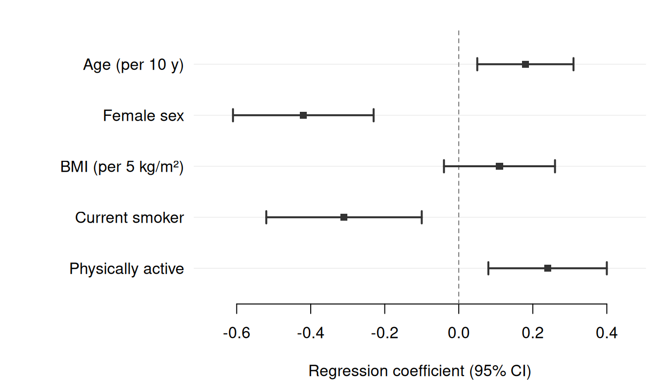
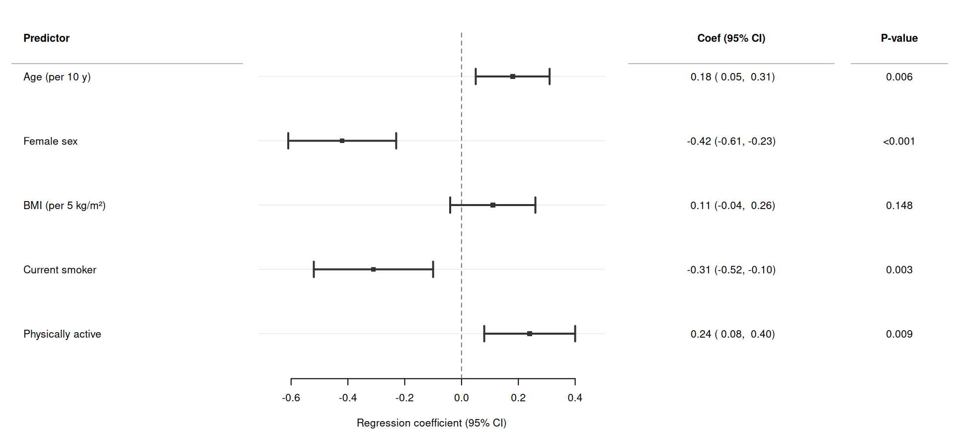
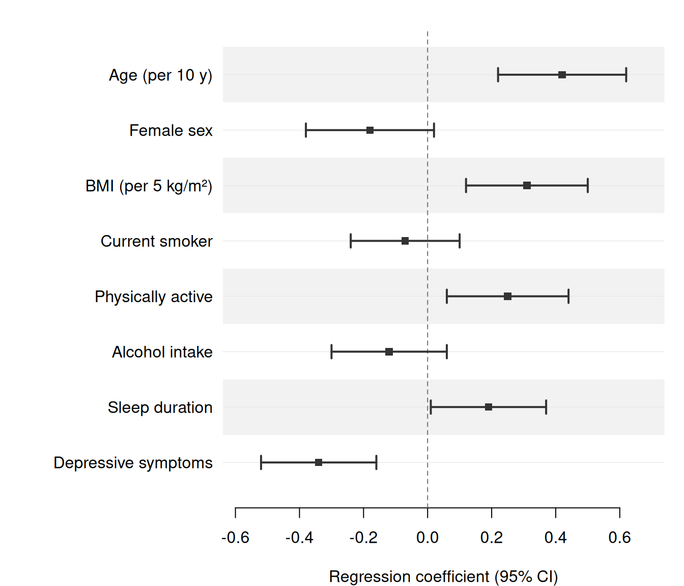
The simplest call requires only three column names: estimate, lower, and upper. Here we display adjusted regression coefficients from a linear model predicting systolic blood pressure (SBP).
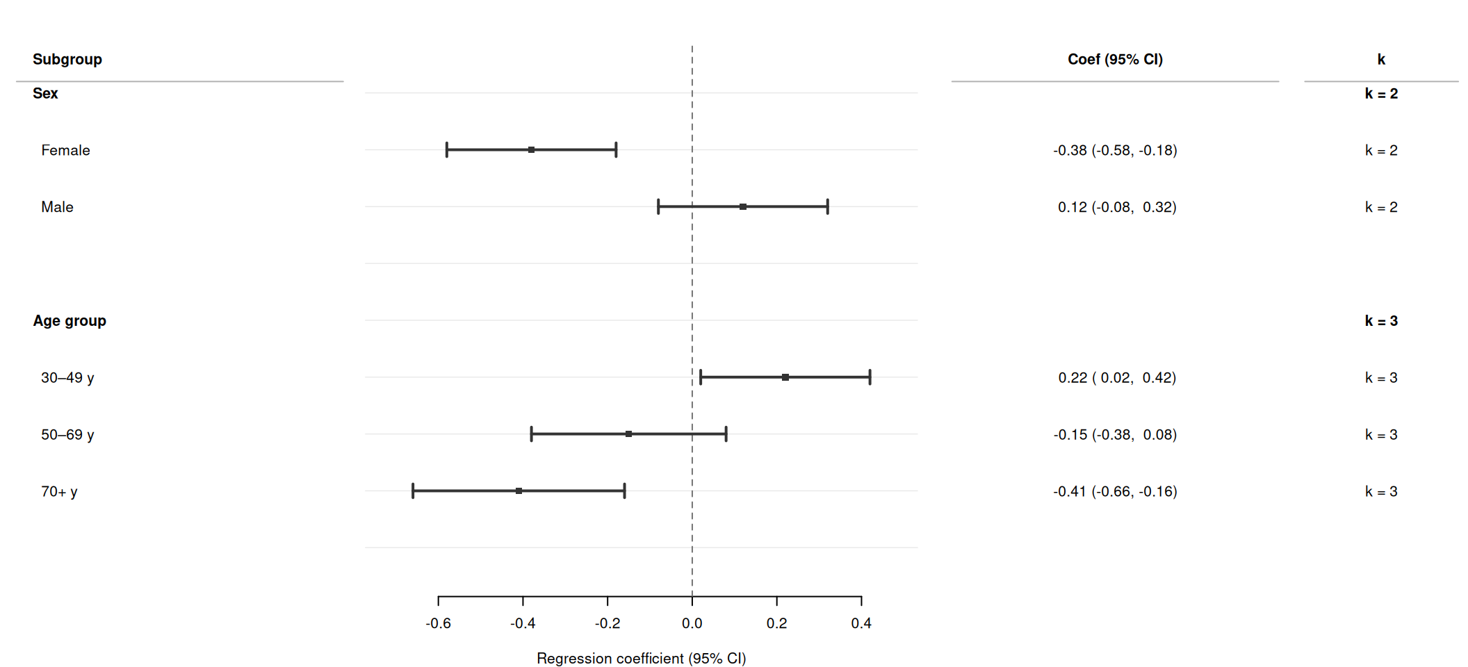
Pass a column name to section to automatically group rows under bold section headers. forrest() inserts a header row wherever the section value changes, indents the row labels within each section, and adds a blank spacer row after each section. No manual data manipulation is required.
Use section_indent = FALSE to suppress automatic indentation, and section_spacer = FALSE to suppress the blank row after each section.
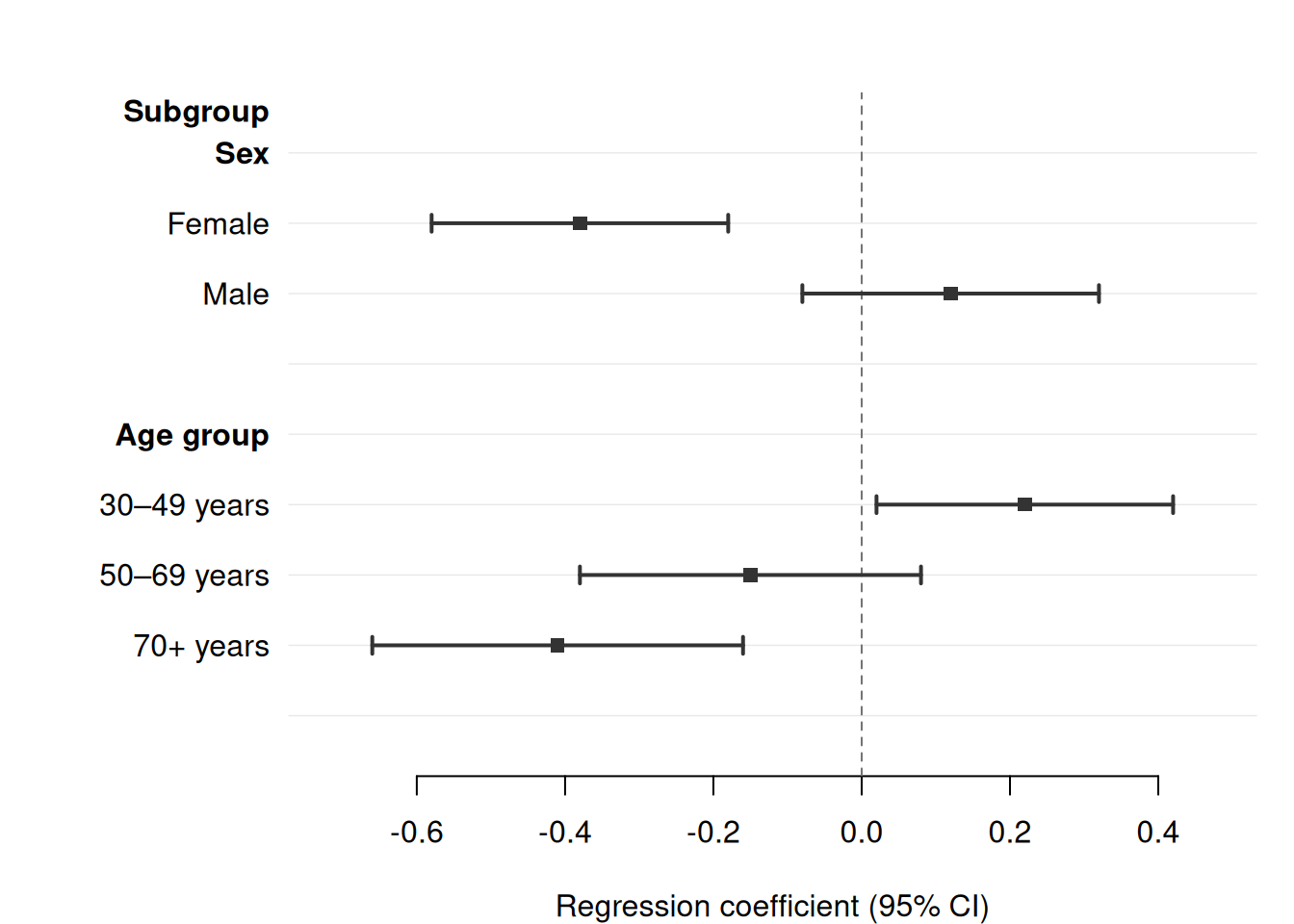
Two-level hierarchy with subsection
For analyses with a nested grouping structure, combine section and subsection. forrest() inserts top-level bold headers for section changes and indented sub-headers for subsection changes within each section.
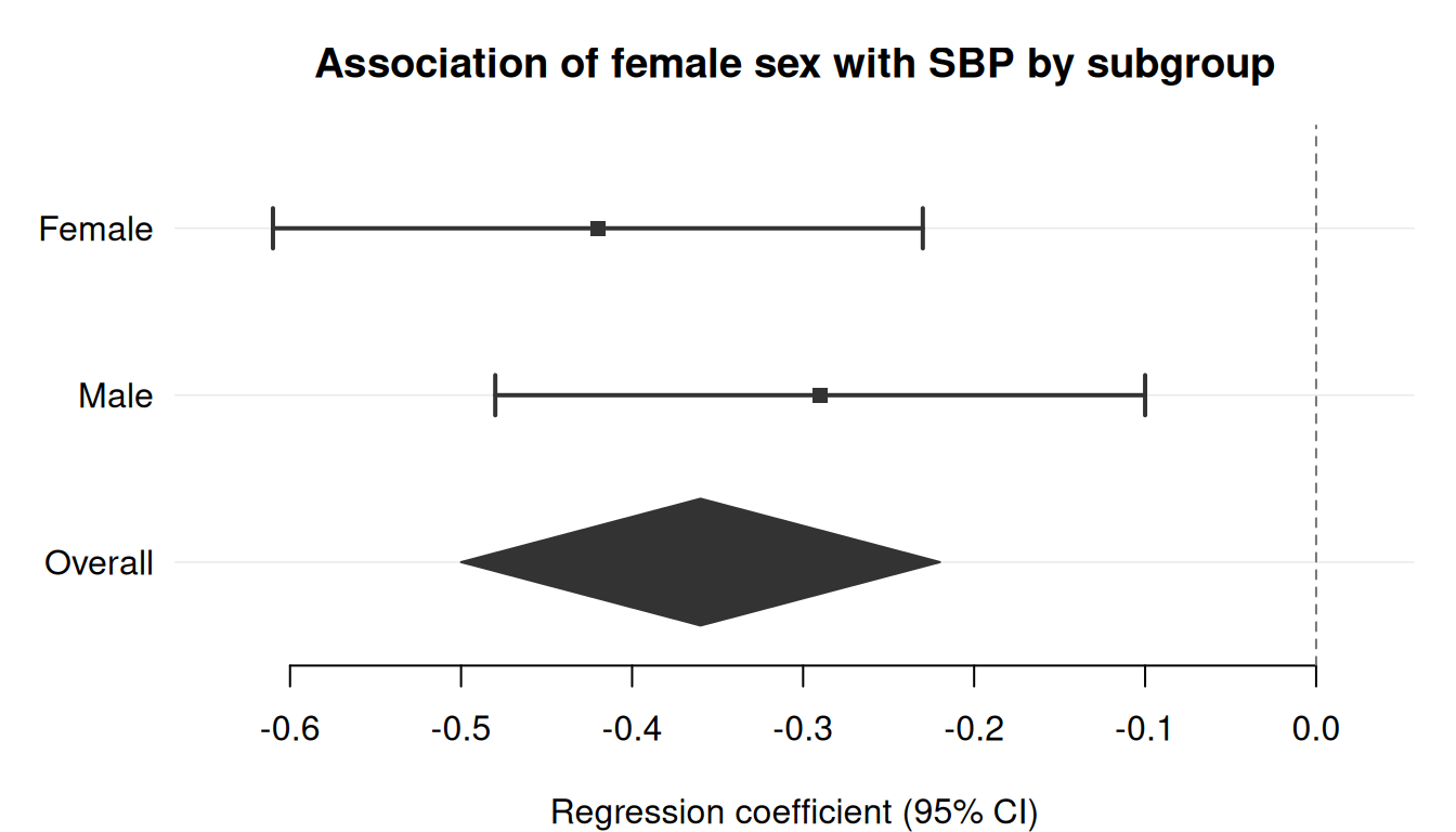
Mark one or more rows with is_summary = TRUE to draw them as filled diamonds instead of squares. This is useful for pooled estimates in meta-analyses or for overall effects after subgroup rows.
sex_dat <-data.frame(label =c("Female", "Male", "Overall"),estimate =c(-0.42, -0.29, -0.36),lower =c(-0.61, -0.48, -0.50),upper =c(-0.23, -0.10, -0.22),is_sum =c(FALSE, FALSE, TRUE))forrest( sex_dat,estimate ="estimate",lower ="lower",upper ="upper",label ="label",is_summary ="is_sum",xlab ="Regression coefficient (95% CI)",title ="Association of female sex with SBP by subgroup")
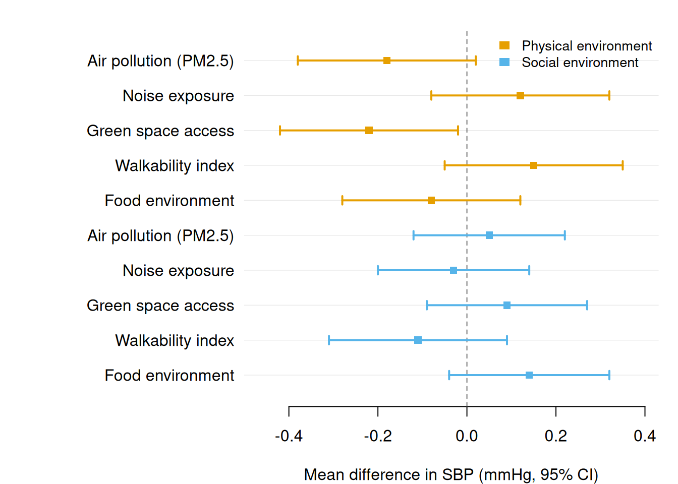
Group colouring
Pass a group column to colour estimates by a categorical variable. A legend is added automatically using the Okabe-Ito colorblind-safe palette.
Set dodge = TRUE (or a positive number) when consecutive rows share the same label value. The CIs are vertically offset within each label band, and the label is displayed once at the group centre. Combine with group to colour the series.
A numeric value for dodge sets the vertical spacing between rows within a group directly (in y-axis units). dodge = TRUE uses the default of 0.25. Structural rows (section and subsection headers, spacers) are always treated as singleton groups and are not affected by dodging.
Wide-format text columns alongside dodged CIs
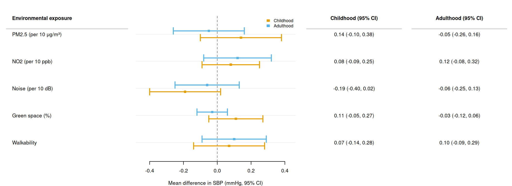
By default, cols text values appear at each row’s dodged y position, keeping them aligned with their CI whiskers. Set cols_by_group = TRUE to collapse each text column to one value per label group — this produces a wide table with one row per label and one column per condition, matching the layout commonly seen in multi-period epidemiology papers.
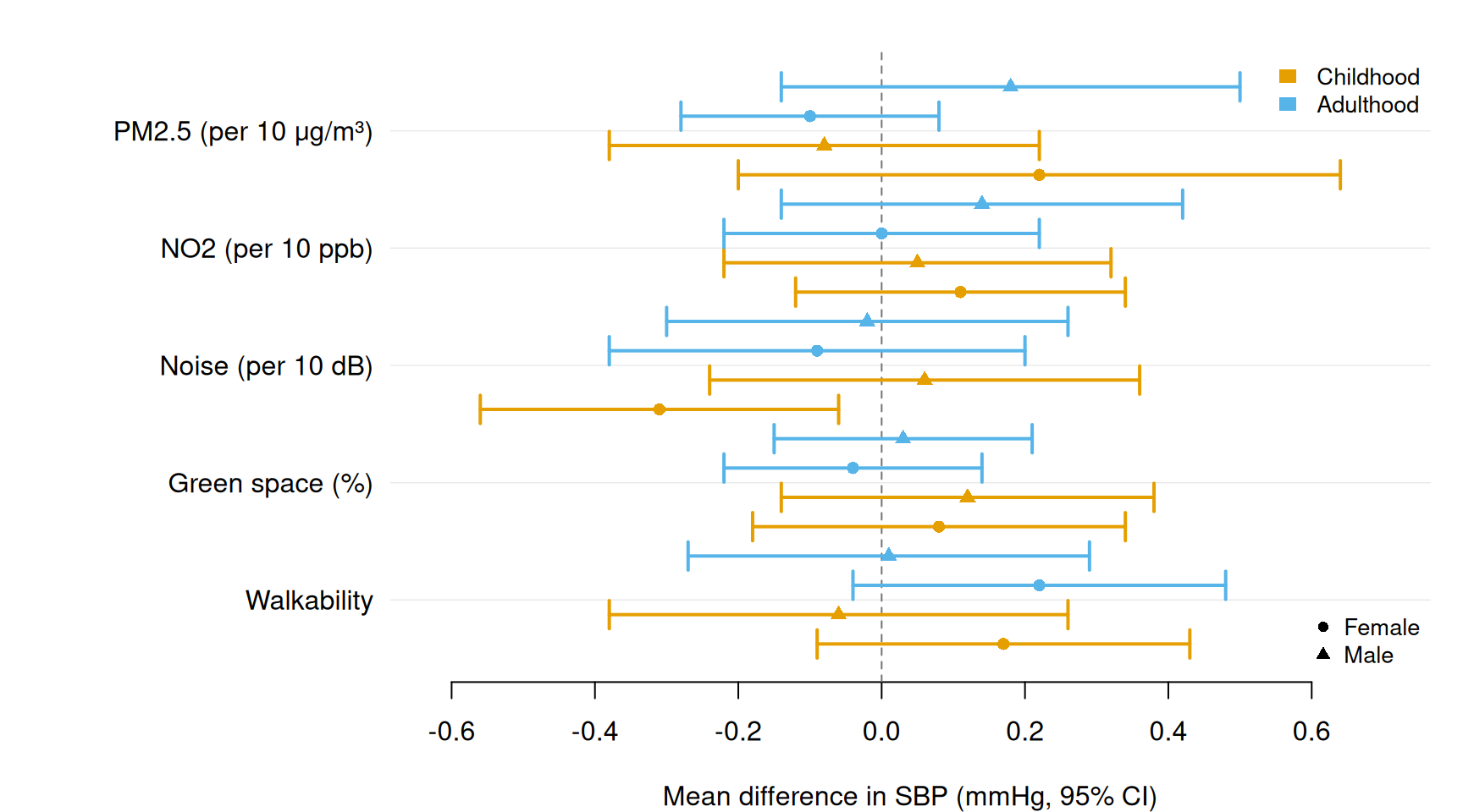
Pass a shape column to assign different point characters per category. Use together with group and dodge to encode two categorical dimensions at once — for example, colour = time period and shape = sex.
When section is active, text columns show "" for section header rows by default. Use section_cols — a named character vector with the same syntax as cols — to populate specific columns in section header rows with a section-level value (e.g. number of studies, total N). The name must match a name in cols; the value is a column in data whose first non-NA entry in each section is used.